JRSSB Paper
% Some results that compare Fox's Laplacian precision matrix (= inv(exponential% covariance) via FEM method%% to%% Higdon's Laplacian precision matrix (= '1st order locally linear')%
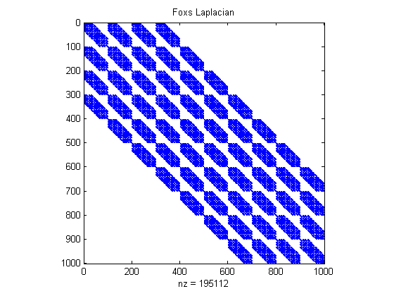
% Using Colin's 3d inv(Exp) using FEMprec% The .25 is 1 over correlation length, Colin says to use 1/4
clear all

[H p]=FEMprec(.25,9);
Omega_fox=H*p*H;  % Precision matrix for prior for phi, phi ~ N(0,constant*inv(Omega_fox))

figure(1);clf
spy(Omega_fox)   % There are 195K non-zeros in this matrix
title('Foxs Laplacian')

% When second param in FEMprec is 9, then A1 is a 1000 x 1000 precision matrix% When second param in FEMprec is k, then A1 is a (k+1)^3 x (k+1)^3 precision matrix
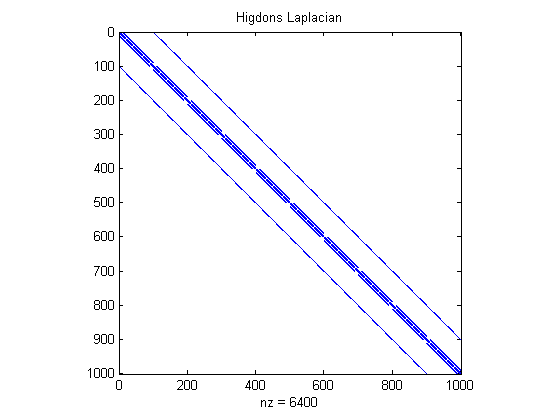
% Using Higdon's 1st order locally linear precision matrix
Omega_hig = GetCovMRFsparse_n3_3d(10,0);  % Another candidate precision matrix for prior for phi, phi ~ N(0,constant*inv(Omega_hig))
figure(2);clf
spy(Omega_hig)   % There are 195K non-zeros in this matrix
title('Higdons Laplacian')
%
Checking BOTTOM face ...Elapsed time is 0.001670 seconds.

Checking SOUTH face ...Elapsed time is 0.003225 seconds.

Checking EAST face ...Elapsed time is 0.009229 seconds.
n = length(Omega_fox)   %1000 x 1000
vert = round(n^(1/3));

%%%%%%%%%%%%%%%%%%%%%%%%%% Now scale the precision matrix by max(A1(:))
Omega_s_fox = Omega_fox/max(Omega_fox(:));
n =

        1000
% Model%% y = F*\phi + \epsilon,%% \epsilon ~ N(0,inv(g_eps*eye(n)))% \phi     ~ N(0,inv(g_phi*Omega))%% The matrix F models the linear measurement process.   Keep it simple for this% exercise, let F trivially be the identity

F=sparse(eye(n));
m=n;
%%%%%%%%%%%%%%%% Posterior for phi = biofilm image | y=noisy image;% phi|y ~ N(g_eps*inv(A)*F'*y, inv(A))
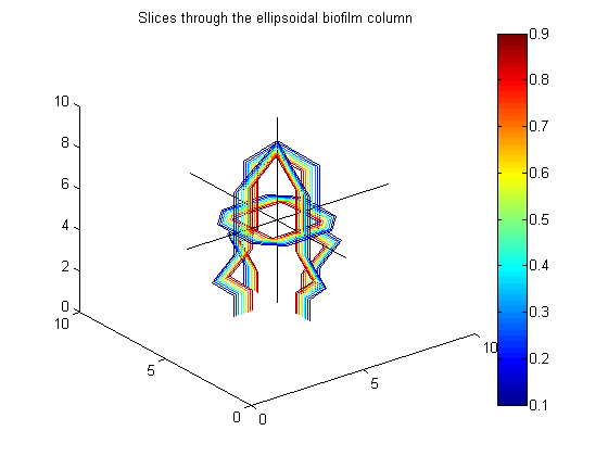
% Posterior precision matrix for p
g_eps = 1;
g_phi = 1;  % Put a lot of weight on prior for a smooth reconstruction
A_fox = g_eps*(F'*F) + g_phi*Omega_s_fox;  % precision matrix of posterior for phi

A_hig = g_eps*F'*F + g_phi*Omega_hig;  % precision of posterior for phi


bio_ellipse = MakeEllipseWFlatBottom([.2 .2 .55]*vert,vert,.3*vert,1);   % An ellipsoidal column of biofilm
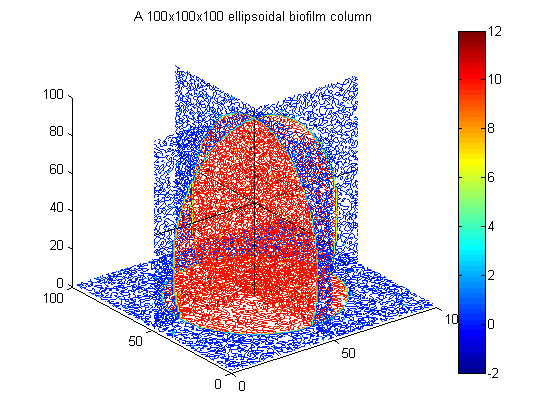
% Example to go in paper
big_vert=100;
big_bio_ellipse = MakeEllipseWFlatBottom([.4 .4 .65]*big_vert,big_vert,.3*big_vert,0);   % An ellipsoidal column of biofilm
figure(20);clf;contourslice(10*big_bio_ellipse+randn(100,100,100),[big_vert/2],[big_vert/2],1);
view(3)
title('A 100x100x100 ellipsoidal biofilm column')
colorbar
hold on
plot3([1 big_vert],[big_vert/2 big_vert/2],[big_vert/2 big_vert/2],'k')
plot3([big_vert/2 big_vert/2],[1 big_vert],[big_vert/2 big_vert/2],'k')
plot3([big_vert/2 big_vert/2],[big_vert/2 big_vert/2],[1 big_vert],'k')
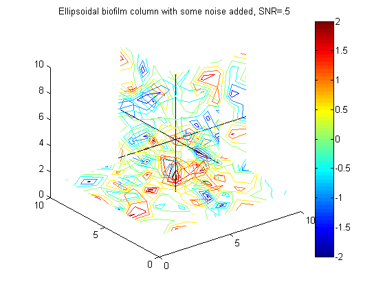
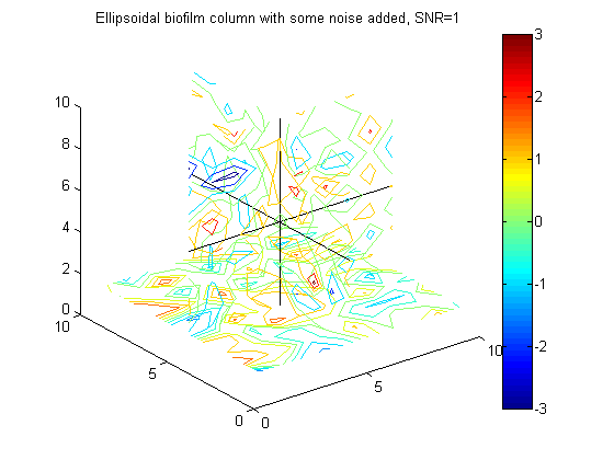
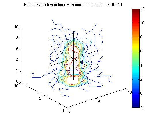
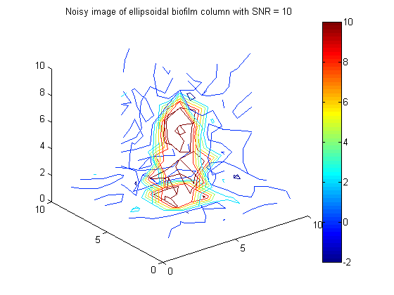
% Generate 10x10x10 image, y = F*phi + \epsilon, where phi is ellipsoidal column of biofilm
y = 10*(F*bio_ellipse(:)) + 1/sqrt(g_eps)*randn(m,1);  % Generate data ....     SNR = 10

figure(6);clf;contourslice(reshape(y,vert,vert,round(m/vert^2)),[vert/2],[vert/2],1);
view(3)
title('Noisy image of ellipsoidal biofilm column with SNR = 10')
colorbar
% Calculate posterior mean for phi using Foxs% Laplacian as prior precision,%

PosteriorMean_fox = A_fox \ (g_eps*(F'*y));


figure(7);clf;contourslice(reshape(PosteriorMean_fox,vert,vert,vert),[vert/2],[vert/2],1);
view(3)
title('PosteriorMean reconstruction of ellipsoidal biofilm column using Foxs Laplacian as prior')
colorbar
hold on
plot3([1 vert],[vert/2 vert/2],[vert/2 vert/2],'k')
plot3([vert/2 vert/2],[1 vert],[vert/2 vert/2],'k')
plot3([vert/2 vert/2],[vert/2 vert/2],[1 vert],'k')

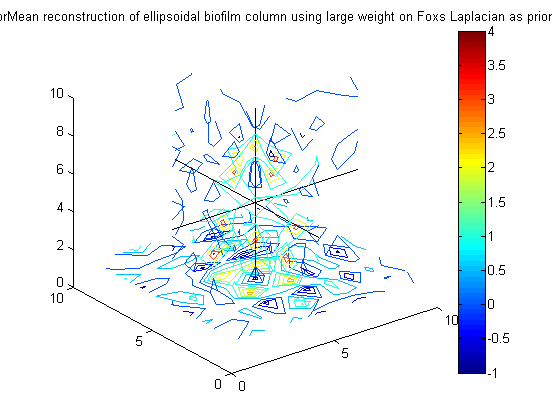
% Get same non-smooth behavior for different values of R = correlation% length and even for large weighting on prior, get

A_fox10 = g_eps*(F'*F) + 10*g_phi*Omega_s_fox;  % precision matrix of posterior for phi

PosteriorMean_fox10 = A_fox10 \ (g_eps*(F'*y));


figure(21);clf;contourslice(reshape(PosteriorMean_fox10,vert,vert,vert),[vert/2],[vert/2],1);
view(3)
title('PosteriorMean reconstruction of ellipsoidal biofilm column using large weight on Foxs Laplacian as prior')
colorbar
hold on
plot3([1 vert],[vert/2 vert/2],[vert/2 vert/2],'k')
plot3([vert/2 vert/2],[1 vert],[vert/2 vert/2],'k')
plot3([vert/2 vert/2],[vert/2 vert/2],[1 vert],'k')
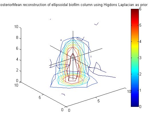
Calculate posterior mean for phi using Higdons Laplacian as prior precision, get smooth reconstruction as anticipated
PosteriorMean_hig = A_hig \ (g_eps*(F'*y));


figure(8);clf;contourslice(reshape(PosteriorMean_hig,vert,vert,vert),[vert/2],[vert/2],1);
view(3)
title('PosteriorMean reconstruction of ellipsoidal biofilm column using Higdons Laplacian as prior')
colorbar
hold on
plot3([1 vert],[vert/2 vert/2],[vert/2 vert/2],'k')
plot3([vert/2 vert/2],[1 vert],[vert/2 vert/2],'k')
plot3([vert/2 vert/2],[vert/2 vert/2],[1 vert],'k')
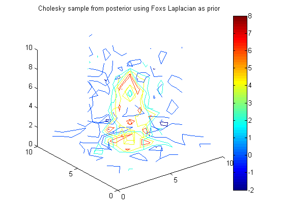
% Get a Cholesky sample
Q_fox = chol(A_fox);   % A = Q'*Q, inv(A) = inv(Q)*inv(Q')
xc_fox = Q_fox\randn(n,1) + PosteriorMean_fox;
vert=round(n^(1/3));
figure(9);clf;contourslice(reshape(xc_fox,vert,vert,vert),[vert/2],[vert/2],1);
view(3)
colorbar
title('Cholesky sample from posterior using Foxs Laplacian as prior')
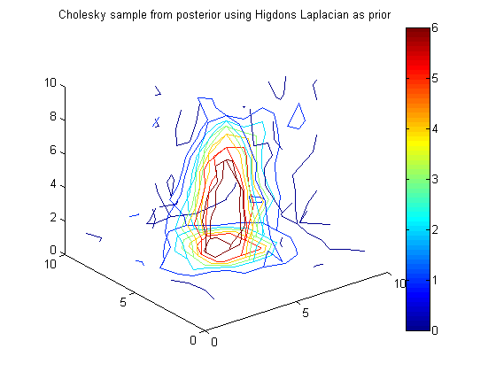
% Get Cholesky samples
Q_hig = chol(A_hig);   % A = Q'*Q, inv(A) = inv(Q)*inv(Q')
xc_hig = Q_hig\randn(n,1) + PosteriorMean_hig;
figure(10);clf;contourslice(reshape(xc_hig,vert,vert,vert),[vert/2],[vert/2],1);
view(3)
colorbar
title('Cholesky sample from posterior using Higdons Laplacian as prior')